1. George Cummings >
2. Artificial Intelligence >
3. Analytical Decision Making >
4. B. Math for Simulations, part 1

B. Math for Simulations, part 1

Previous: Optimization

As mentioned before, these posts are my aide-memoires. They do not replace the course slides, but present some additional notes that may help understand the theory behind the techniques.

B.1. Discrete Math Concepts

B.1.1 Random Variable (r.v.)

An r.v. is a mapping of all possible outcomes in a sample space to real numbers. ¹ Its actual value is uncertain because it is, well, random. For example, a sample space for the possible results of a coin toss {heads, tails} maps to the random variable: $$ \color{#515151}{ X(ω) = \begin{cases} -1, & \text{if}\ ω = heads \\ 1, & \text{if}\ ω = tails \end{cases} } $$

A sample space for the effectiveness of a company of soldiers in a World War II battle simulation {Suppressed, Neutralized, Effective} could map to the random variable: $$ \color{#515151}{ X(ω) = \begin{cases} -1, & \text{if}\ ω = Neutralized \\ 0, & \text{if}\ ω = Suppressed \\ 1, & \text{if}\ ω = Effective \end{cases} } $$

In the example of the Poisson Distribution below, the r.v. would be X = {0, 1, 2, …, ∞}, i.e. positive integers, with no upper bound.

A random variable does not look like the variables that we learned about in middle school algebra, e.g. a single real number such as x = 5.3. A random variable is more like x = “I dunno, but it’s going to be a value from the set {…}, and here are the probabilities for each value.”

B.1.2 Distributions and Uniform Distribution

B.1.2.1 Frequency Distributions

A frequency distribution describes the number of observations for each possible outcome of an r.v. ² For example, say apple is mapped to 2, banana is 3, and grape is mapped to 4. We’ll throw in “nothing” as well. Its r.v. for fruit selection is: $$ \color{#515151}{ X(ω) = \begin{cases} 1, & \text{if}\ ω = nothing \\ 2, & \text{if}\ ω = apple \\ 3, & \text{if}\ ω = banana \\ 4, & \text{if}\ ω = grape \end{cases} } $$

A possible frequency distribution could be f(X) = [4, 5, 3, 9], meaning that apples were selected five times, bananas three times, and grapes nine times. “Nothing” was selected four times.

B.1.2.2 Probability Distributions

A probability distribution is an idealized probability frequency distribution ³. Probability, because each outcome’s value is a probability (a value between 0 and 1) that it will be selected in a single test. Idealized, because the set of probabilities adhere closely enough to well-known patterns of random behaviour.

Take the example above where apples are mapped to 2, etc. It could be shown by Grocer Martha from her sales history that the frequency distribution for the last month was f(X) = [235, 1349, 5487, 2304], assuming her rather strict rule that a customer could choose only one of those fruits per visit. The naive probabilities of the next customer selecting nothing, apples, bananas, or grapes are thus: X = [0.0251, 0.1439, 0.5852, 0.2458]. This means that, judging from history, there is a good chance that in any given visit, the customer will choose the bananas.

However, this is not a probability distribution because it is neither random behaviour nor is it idealized. A probability distribution follows the observation that blind, random selections follow certain patterns.

One such pattern is the uniform distribution: all outcomes are equally likely, for example a blind selection of fruits. The uniform distribution of the r.v. X = {0, 1, 2, 3} would be [0.25, 0.25, 0.25, 0.25]. Coin tosses have the uniform distribution [0.5, 0.5]. If you plotted the results of a uniform distribution on a graph, you would get a straight, horizontal line.

Other probability distribution plots look like the famous “bell curve,” where most outcomes are close to the expected behaviour (the median, if you will), and rarer outcomes are further away. Two such probability distributions are the Binomial and Poisson distributions.

B.1.3 Binomial Distribution

A binomial distribution is the probability distribution of one of two possible outcomes over a series of trials such as a series of coin tosses, i.e. the r.v. is X = {0, 1}. Formally: $$ \color{#515151}{ P_x = (^n_x)p^xq^{n-x} } $$ where

• n is the number of trials
• x is the number of times a specific outcome is being tested
• p is the probability of success on a single trial
• q is 1 - p, the probability of failure on a single trial.
• \( \color{#515151}{ (^n_x)} \) is a combination. \( \color{#515151}{ (^n_x) = {n! \over x!(n-x)! }} \)

Take all the possible values of x informed by p over a series length n, and you have the distribution. If graphing that distribution:

• If p = 0.5 (even odds), the graph looks like a bell curve, with the x-axis defined by the number of successes and the y-axis defined by Px. If there are four trials, the top of the curve is at 2 successes. For 12 trials, the top of the curve will lie at 6 successes.
• The distribution curve for p = 0.7 (e.g. the coin is unfair) will shift to the right.

B.1.4 Poisson Distribution

A particular set of probabilities of the number of arrivals over some fixed period of time given an already established average, called the arrival rate.

Say the records show that an average of 80.6 customers show up at Gille’s lunch counter in downtown Montreal every hour between 11:30am and 1:30pm Monday to Friday. Gerald has errand to run tomorrow. What is the probability that more than 45 people show up tomorrow (Friday) between 12pm and 12:30pm when Gerald has to go the bank and leave his station unmanned? You might need someone else on shift. Use a Poisson Distribution since you are dealing with people. Notice that although the average is a continuous number, the arrivals are discrete numbers.

The set of outcomes will be the r.v. X = {0, 1, …, 100}, since we really do not think that more than one hundred customers will show up in the given half hour, even taken to extremes. This is borne out by Poisson Distributions anyway.

The probability of any one number in the r.v. being selected is calculated formally: $$ \color{#515151}{P(X = x) = e^{-\lambda}\lambda^x \over x!} $$ where

• P(X = x) means “Probability of a single selection taken from the random variable turning out to be x.
• x is the number of occurrences. Unlike the binomial distribution, x is not limited.
• X is the random variable, the set of possible outcomes. Since it depends on x, which has no set limit, it is the set of all possible outcomes from 0 to infinity.
• e is the Euler constant, 2.718…
• λ (lambda) = Var(X), or the variance of the expected value of X (this is the arrival rate). Forget variance for now: it can be estimated by the average rate at which events occur. Say five people show up every hour. Then λ = 5. If five people show up every two hours, then λ = 2.5

Let’s punch in the values…

• X = {0, 1, …, ∞}
• e = 2.718…
• λ = 80.6/2 = 40.3. # The unit is half an hour
• If x is exactly 45, then the probability P(X=45) is $$\color{#515151}{\frac{2.718^{-40.3}40.3^{45}}{45!} ≈ 0.0456 } $$
• If x = 47, then the probability P(X=47) is $$\color{#515151}{\frac{2.718^{-40.3}40.3^{47}}{47!} ≈ 0.0342 } $$

Punching these in on a desktop calculator is pretty painful. Python’s scipy module has a poisson function that makes it easy. The instructions use µ instead of λ, since lamba is reserved in Python.

from scipy.stats import poisson

mu = 40.3  # Average customers per half hour unit.
k = 45  # What's the probability?

print(round(poisson.pmf(k, mu), 4))  # Probability Mass Function
0.0456

As for “more than 45,” one can simply add up each probability to get the answer under the curve.

from scipy.stats import poisson

for x in range(45, 81):
    probability += poisson.pmf(x, mu)
print(round(probability, 4)
0.2494

Hmm. A 1 in 4 chance that Gerald’s absence will be felt. No need to put on any more staff.

Not noticeable in this simple code is the diminishing probability as x moves away from λ. Setting the upper bound to 100 instead of 80 does not add any appreciable difference. We can see this in a representation of Poisson distributions in a graph:

import matplotlib.pyplot as plt
import numpy as np

customermin = 45
x = np.arange(0, 100)
y = poisson.pmf(x, mu=40.3)
colours = [1]*customermin + [4]*(100-customermin)
plt.scatter(x, y, c=colours, cmap='coolwarm')
plt.show()

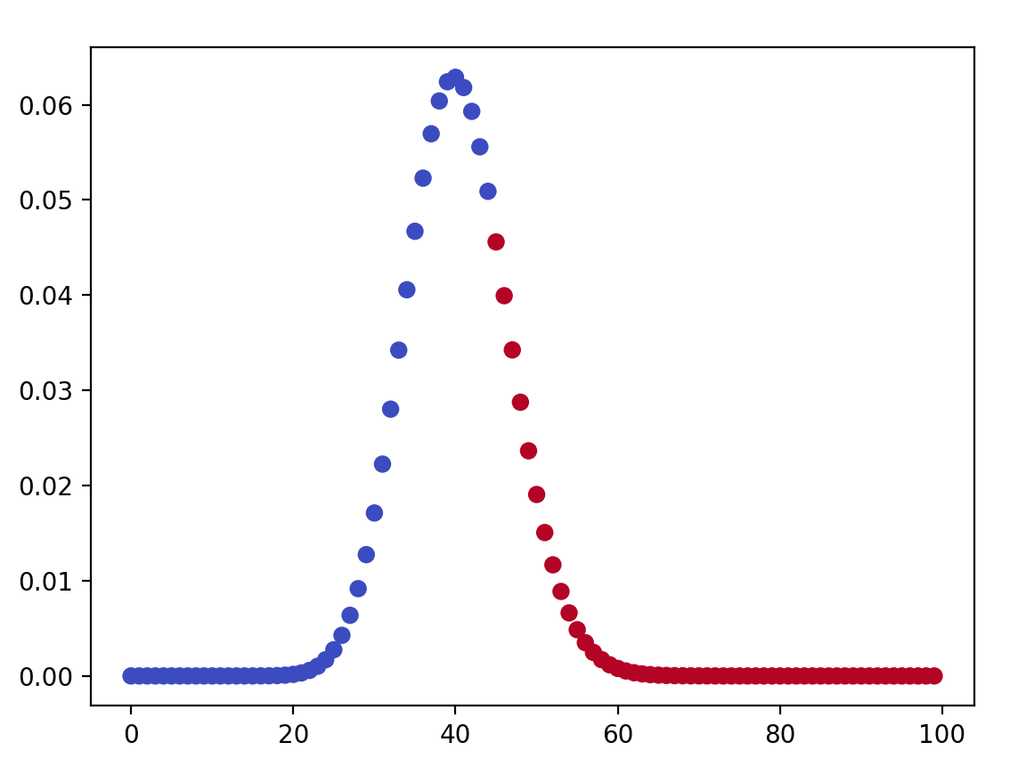
And so on. See the graph? The Poisson distribution looks like a binomial distribution at p=0.5, i.e. a bell curve, but it is centered on λ = 40.3, rather than x/2 = 50.

Next post will discuss the continuous probability distribution called Normal Distribution, and some math prerequisites to understand it.