Basic Calculus for AI
Machine Learning is the art and science of getting computers to generate models, functions that describe how certain phenomena affect other phenomena. These models can be used to predict results from what-ifs given to them by a user.These models are refined (the learning part of Machine Learning) by measuring their accuracy. However, since there will always be unavoidable errors in the models, the machine learning mechanism needs to know when to stop training its model because it just won’t get any better. To do this, it needs to know the idea of minimum. And the idea of minimum can be taught to a computer efficiently through calculus! Not only this, but the computer can be taught how dramatically it needs to alter its model-training cost functions to get to the minimum error.
A.1. Single Variable Functions
A.1.1 What is a function?
A function is a mathematical expression with one or more variables. A variable is a label representing any quantity. Programmers are pretty keen on functions. The math function \(f(x, y) = x+y\) can be programmed thus:
def f(x, y):
  """Simple addition"""
  return x + y

print(f(2, 3))
5
A single-variable function is just what is says on the can, for example the parabola defined by \(f(x) = 20x^2 + 5x + 3\):
def f(x):
  """A parabola with predefined coefficients"""
  return 20*(x**2) + 5*x + 3
A.1.2 Derivatives
A derivative calculates the rate of change of a single-variable function. Take the fable1 of boiling frogs: the idea was that one can cook a frog to death if the temperature of the water that it is in is raised slowly enough not to be detected. If the rate of change is too high, the frog figures out what is happening and hops out of the pot.
Say someone measured the temperature of a pot of water (and the frog) over 10 minutes and plotted the results on a graph. Time in seconds is the x-axis. Temperature, a variable dependent on time, is the y-axis [i.e., f(x)]. From machine-learning magic, the computer discovered the best-fitting function to the data was a sigmoid function2:
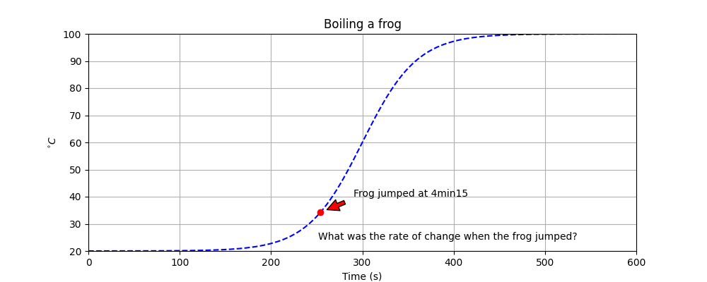
The moment the frog jumpied out is indicated at a point in time. By calculating the rate of change (and repeating the experiment of course), one can issue a warning, “do not raise the temperature faster than y degrees per second.”
It doesn’t matter here that the frog jumped at 35°C. It mattered that the temperature was rising noticeably. What was the rate?
A.1.2.1 Mathematically defining the derivative
- A line is a series of points (x, y) connected by a straight path, stretching in both directions to infinity.
- A slope is the steepness of a line.
- A secant is a line that crosses a curve twice.
- A tangent is a secant, created from two points infinitesimally close to each other on the curve.
- A derivative is the slope of a tangent.
A.1.2.2 The Line
A line is a series of points (x, y) connected by a straight path, stretching in both directions to infinity. Its equation is: \(y = mx + b\), where m is the slope (discussed below) and b is the y-intercept: where the line crosses x = 0.
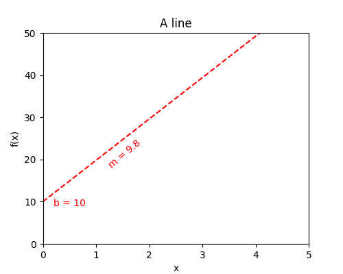
In this case, b = 10, and the slope (m) is 9.8. The equation is then \( y = 9.8x + 10\).
Smart math people will recognize \( y = mx + b\) as an incredibly simple polynomial.
A.1.2.3 The Slope of a Line
Draw a line through two points, \(P0(x_{0}, y_{0})\) and \(P1(x_{1}, y_{1})\).
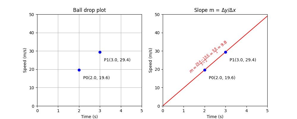
A slope describes the direction and steepness of a line, in this case 9.8. It is found through the simple equation: \(m={\Delta y \over \Delta x}\), which is a fancy way of writing \(m={{y_1 - y_0}\over{x_1 - x_0}}\).
- A positive number means the line is bottom-left to upper-right. For example, increasing profit over time.
- A negative number means the line is upper-left to bottom-right. For example, decreasing cognitive ability over the course of MMAI (haha just joking).
- The greater the value, the steeper the line.
A.1.2.4 Secant of a Curve and the Average Rate of Change of a Curve
Take a simple curve with the equation \( y = x^2\).
A secant is a line that intersects a curve twice.
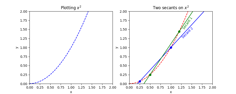
The average rate of change between two points (\(m_{PQ}\)) along a curve is a secant slope.
The equation for this is:
$$ m_{PQ} = {{f(x) - f(a)}\over{x-a}} $$
where
- P and Q are the first and second points on the curve, respectively
- x is \(x_1\) and a is \(x_0\)
- Likewise, f(x) is \(x_{1}\) and f(a) is \(y_{1}\).
Basically, this equation is the same as the slope of a line, \(m = {\Delta{y}\over\Delta{x}}\)!
I’ll use y and f(x) interchangeably through the rest of this post because, for single-variable functions, \(y=f(x)\).
A.1.2.5 The Slope of the Tangent of a Curve at a Given Point
The slope of a curve at a given point, the tangent slope, is not actually a slope of a curve with one given point. By definition, you cannot have a slope with just one given point. You need two points.
However, it can be calculated as if there was only point, because all one does is calculate the slope of a secant created from two points on the curve that are really, really, really close to the given point.
To show that the two points are really, really, really close to each other we add the infamous notation \(\lim_{a \to x}\) to the \(m = {{f(x) - f(a)}\over{x -a }}\) slope equation. This notation means that a is unbelievably, horrifyingly, infinitesimally close to x, almost … but … never … quite … touching:
$$ m_{pq} = \lim_{a \to x}{{f(x) - f(a)}\over{x - a}} $$
The other way of stating the same thing is by representing the first value of the secant with x instead of a (i.e., \(x_0\)) and then introducing h as a tiny, tiny, tiny increase of x: \(x + h = x_1\). This expression is useful because one can use it to calculate the derivative algebraically.
$$ m_{pq} = \lim_{h \to 0}{{f(x + h) - f(x)}\over{h}} $$
Notice that PQ is now pq? It means that the distance between points P and Q is horribly small. Additionally, using lim can be unwieldy, so often we use \(m_{pq} = {{\Delta y}\over{\Delta x}}\) instead, but this time replacing the (\(\Delta\)) with the simple latin d to demonstrate \(lim_{a \to x}\).
$$ m_{pq} = {{dy}\over{dx}} $$
A.1.2.6 Derivatives
Guess what! A derivative is just the calculus way of saying “the slope of the tangent.”
Let us find the derivative of \(f(x)=3x^5\).
$$\begin{aligned} f’(x) &= \lim_{h \to 0}{{f(x + h) - f(x)}\over{h}} \\ f’(x) &= \lim_{h \to 0}{{3\color{green}{(x + h)^5} - 3x^5}\over{h}} \\ f’(x) &= \lim_{h \to 0}{{\color{green}{3}(x^5+5x^4h+10x^3h^2+10x^2h^3+5xh^4+h^5) - 3x^5}\over{h}} \\ f’(x) &= \lim_{h \to 0}{{\color{red}{3x^5}+15x^4h+30x^3h^2+30x^2h^3+15xh^4+h^5 - \color{red}{3x^5}}\over{h}} \\ f’(x) &= \lim_{h \to 0}{{15x^4\color{green}{h}+30x^3\color{green}{h^2}+30x^2\color{green}{h^3}+15x\color{green}{h^4}+\color{green}{h^5}}\over{h}} \\ f’(x) &= \lim_{h \to 0}{{\color{red}{h}(15x^4+30x^3h+30x^2h^2+15xh^3+h^4)}\over{\color{red}{h}}} \\ f’(x) &= \color{red}{\lim_{h \to 0}}15x^4+30x^3h+30x^2h^2+15xh^3+h^4 \\ f’(x) &= 15x^4+30x^3(0)+30x^2(0)^2+15x(0)^3+(0)^4 \\ f’(x) &= 15x^4 \end{aligned}$$
Man, that’s a lot of arithmetic. But notice! The derivative of \(3x^5\) is \(15x^4\). This is an example of the power rule, which is \(f’(x) = n\times f(x)^{n-1}\), i.e.:
- Multiply each element’s coefficient by the value of its exponent
- Subtract each element’s exponent by 1.
For example, take the polynomial \( f(x) = 5x^{2} + 5\):
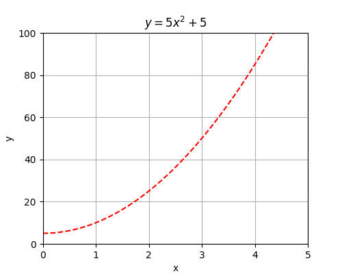
The derivative (dy/dx) of a function f(x) is denoted f’(x). We calculate its derivative thus:
$$\begin{aligned} f(x) &= 5x^2 + 5 = 5x^2 + 5x^0 \\ f’(x) &= (2 \times 5)x^{2 - 1} + 0 \times 5x^{0 - 1}\\ f’(x) &= 10x^1 + 0 \\ f’(x) &= 10x \end{aligned}$$
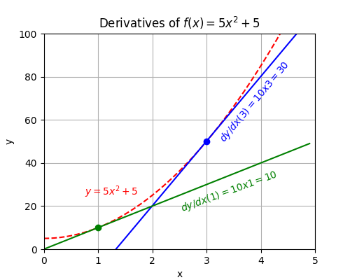
This means, given a curve with the equation \(y = 5x^2 + 5\):
| x | f(x) | f’(x) |
|---|---|---|
| 1 | \(5 \times 1^2 + 5 = 10 \) | \(10 \times 1 = 10\) |
| 3 | \(5 \times 3^2 + 5 = 50 \) | \(10 \times 3 = 30\) |
A.1.2.7 Conclusion
- A line is a series of points (x, y) connected by a straight path, stretching in both directions to infinity.
- A slope is the steepness of a line.
- A secant is a line that crosses a curve twice.
- A tangent is a secant, created from two points infinitesimally close to each other on the curve.
- A derivative is the slope of a tangent.
Now look at that boiling frog example above. Don’t worry about its derivative. Just contemplate rate of change.
A.2 Detecting maximums and minimums
Everyone knows what maximums and minimums are. Maximum speed = speed that one cannot (legally) surpass. Minimum wage = an employer cannot pay an employee less than this. Mathematically, a function has a maximum or minimum where the dependent variable y plateaus, and (just as importantly), reverses its direction.
A.2.1 Detecting a maximum at point x
- \(lim_{n \to x}f(x-n)\) has a positive slope. This is discovered by differentiation, that is to say the calculation of the derivative at that point, i.e., \(lim_{n \to x}f’(x-n)\).
- The plateau is detected when the derivative of the function at point x is 0.
- The decrease is detected if \(lim_{n \to x}f’(x+n) < 0\).
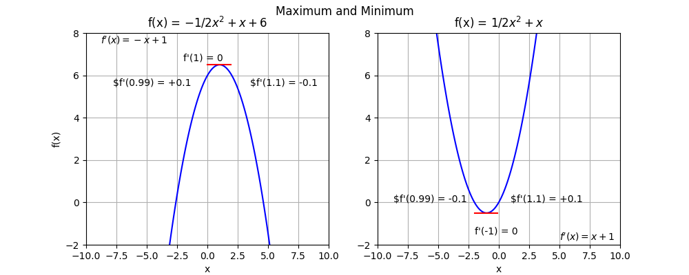
A.2.2 Detecting a minimum at point x
The opposite is true for minimums:
- \(lim_{n \to x}f’(x-n) < 0\).
- \(f’(x) = 0\). Just like for the maximums.
- \(lim_{n \to x}f’(x+n) > 0\).
Note that if one reaches a plateau, and then f(x) continues in the same direction without reversing, no maximum or minimum was reached.
Here is a little demo program:
#!/usr/bin/env python3
"""
Demonstrating detecting the minimum.

By using slopes, one can find if a minimum has been reached
without comparing every ... single ... variable in a range
with all the others.
"""

import numpy as np

def f(x):
    """A parabola with fixed coefficients"""
    return 0.5*x**2 + x

def f_prime(x):
    """The derivative of the parabola"""
    return x + 1

def start():
    """
    Simulate a model being trained

    Learning rate n = 0.1 with an array of x
    from -3.0 to 3.0. The errors E are simulated by
    f(x).
    """"
    X = np.arange(-3.0, 3.0, 0.1)

    # Use round() to deal with Python floating pt
    for i in range(len(X)-1):
        x = round(X[i], 1)
        slope = round(f_prime(x),1)
        if slope == 0 and f_prime(round(X[i+1],1)) > 0:
            print(f"Minimum found at f({x})")
            break

start()
Minimum found at f(-1.0)
A.2.3 Local and absolute maximums and minimums
Should a function have a series of peaks and valleys, then the absolute maximum will be the tallest peak of all the peaks. Likewise, the absolute minimum is the deepest of all the valleys.
A local maximum and local minimum is merely one of those series of peaks and valleys.
Formally:
- Let c be a number in a domain. For all x in that domain, if f(c) > f(x) then f(c) is the absolute maximum.
- Let c be a number in a domain. For all x in that domain, if f(c) < f(x) then f(c) is the absolute minimum.
Absolute maximums and minimums are used in AI optimization problems. Local maximums and minimums are important later on in AI in Finance: local maximums on either side of an absolute maximum in stock price is a buy/sell trigger.
The Next Stuff
The next post will deal with concepts related to multi-variable functions:
- Level Curves
- Linear Approximation
- Partial Derivatives
- Differential Partial Derivatives
- Directional Derivatives
- Lagrange Multiplier
- The Most Important Thing to Understand DL: the Chain Rule