Basic Calculus for AI, part 2
So far, we have been dealing with just two dimensions: x and its dependent variable f(x). What about three-dimensional problems where the function takes two variables, i.e. \(f(x, y)\), and returns a third? Or a five-variable function that returns a sixth?A.3 Multi-variable Functions
A.3.0 Some Preliminaries
R-notation
In discrete math, a two-dimensional set is described as \(\mathcal{R}^2\) and a one-dimensional set is described \(\mathcal{R}\). An expression \(z = ax + by + c\) belongs to the three-dimensional set, \(\mathcal{R}^3\).
Slopes vs Gradients
Consider a simple 3D function. The derivative of a 3D object is called the gradient of the tangent plane rather than the slope of the tangent, because the derivative of a 3d object is a plane, not a line.
A.3.1 Level Curves
Think of a contour line on a topographic map: the latitude and longitude of each point on the contour are all over the place, but altitude remains the same. This is an example of a level curve.
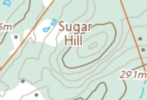
A level curve of a 2-variable function is a curve that is formed by a subset of its points that share a constant in z. For any value of n where \(f(x_n, y_n) = 5\), its point has a gradient zero, and it forms part of a level curve because it shares the constant 5. This will be important in the next post when dealing with Lagrange Multipliers.
A.3.2 Linear Approximation and the Tangent Equation
Linear approximation is used to demonstrate that adding two perpendicular slopes together to come up with a multi-variable rate of change does not add any significant error.
A.3.2.1 Tangent Equation
We already explored the tangent slope. The tangent equation is the same as any linear equation: \(y = mx + b\). The slope (m) we can find from the derivative. The y-intercept (b) we can find from the point (i.e. the two points really, really, really close to each other).
The equation of a tangent of f(x) at a given point (a,f[a]) (i.e. a constant) is
$$ y = f(a) + f’(a)(x-a) $$
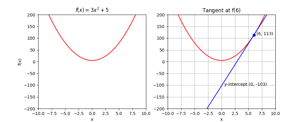
So take a curve, say \(f(x) = 3x^2 + 5\). Its derivative is \(f’(x) = 6x\). We want to know the the equation of the tangent at x = 6.
$$\begin{aligned} f(6) &= 3\times6^2 + 5 = 113 \\ f’(6) &= 36 \\ y &= 113 + 36(x-6) \\ y &= 113 + 36x - 36\times6 \\ y &= 36x - 103 \\ \end{aligned}$$
A.3.2.2 Linear approximation using the tangent equation
Linear approximation is the use of a tangent equation to estimate the location of another point on the curve. The closer to points are to each other (i.e. \(\lim_{x_1 \to x_0})\), the more the curve between those points looks like the tangent, and the more accurate the estimate. The further away the points, or the curvier the curve, then the tangent diverges more and the estimate becomes less accurate. The error in estimation is denoted \(\epsilon\).
A.3.2.3 Practical linear approximation
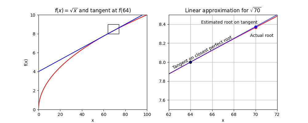
To borrow an exercise from Calc Workshop, let’s use linear approximation to estimate the square root of 70:
Step One: Identify the function and derivative
- \(f(x) = \sqrt{x}\)
- \(f’(x) = {1\over2}x^{-{1\over2}} = {1\over2\sqrt{x}}\)
Step Two: Create the tangent equation for a known square
- We find the closest perfect square, \(a = 64\).
- \(f(64) = 8\)
- \(f’(64) = {1\over2(8)} = {1\over16}\)
- The tangent line equation is \(y = f(a) + f’(a)(x-a)\), so \(y = 8 + {1\over16}(x-64)\).
Step Three: Make the estimate
Replace x with the actual value for which we want the square root: \(y = 8+ {1\over16}(70-64) = 8 + {1\over16}(6) = 8.375 \)
Saieth the calculator: 8.367. A close estimate, off by \(\epsilon = 0.008\).
 |
|---|
To repeat: linear approximation is used to demonstrate that adding two perpendicular slopes together to come up with a multi-variable rate of change does not add any significant error. Why? Because at the scale of the small differences between the points that form the tangents, infinitely small errors + infinitely small errors = infinitely small error.
A.3.3 Partial Derivatives
The derivative of a multi-variable function can be broken down into partial derivatives. A partial derivative is the derivative of a function where all variables but one have been “frozen” into a constant.
$$ dz = {\delta{f}\over\delta{x}}dx + {\delta{f}\over\delta{y}}dy $$
Partial derivatives use the lower-case delta (\(\delta\)) instead of d. The partial derivative with respect to x can also be notated \(f_x\) and the partial derivative with respect to y can be notated \(f_y\).
$$ f’(x,y) = f_x + f_y $$
Calculation
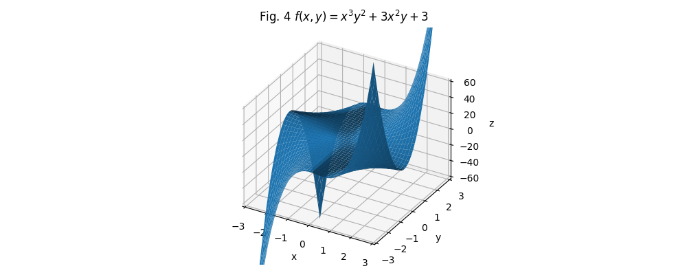
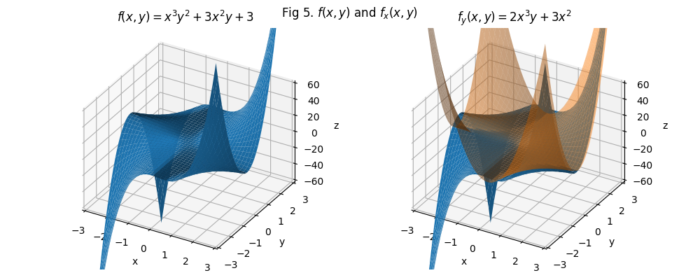
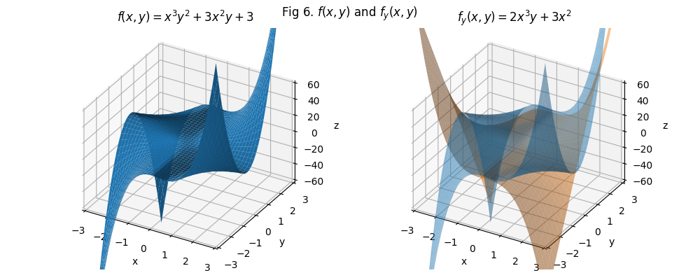
Say \(f(x,y) = x^3y^2 + 3x^2y + 3\). I just wrote it down off the top of my head. Its 3D projection looks like this:
Step one: partial derivative with respect to x
- Freeze all y and their exponents by replacing them with constants:
- a replaces \(y^2\)
- b replaces \(y\)
- \(f(x,y) = ax^3 + 3bx^2 + 3\).
- The partial derivative is \(f_x = 3ax^2 + 6bx\)
- Put the y’s back: \(f_x = 3x^2y^2 + 6xy\)
Step two: partial derivative with respect to y
- Freeze all x and their exponents by replacing them with a constants:
- c replaces \(x^3\)
- d replaces \(x^2\)
- \(f(x, y) = cy^2 + 3dy + 3\).
- The partial derivative is \(f_y = 2cy + 3d\)
- Put the x’s back: \(f_y = 2x^3y + 3x^2\)
Once you feed constants into those partial derivative formulae, you will have the rate of change in the x- and y- axes. However, the world doesn’t work in just the x- and y- axes. Sometimes one wants to know the rate of change at a certain point at, say, 34 degrees from optimal. Enter directional derivatives and the gradient vector!
Next Up
Next post goes off on an angle. Here are the remaining calculus topics…
- Vectors and Unit Vectors
- Gradient Vectors
- Directional Derivatives
- Lagrange Multiplier
And …
- The Chain Rule