Basic Calculus for AI, part 4
This post continues with a complicated subject, Lagrange Multipliers. The good news is that there are quite a few resources on the Web that explain the concepts, so that all I need to do here is sum up.A.5 Lagrange Multiplier
Sometimes one does not need to find an absolute minimum or maximum for a function. One may wish to put a constraint. For example, if profit is calculated with \(f(resource_0, resource_2)\), there may be a constraint that the budget for the resources is \(resource_0 + resource_1 = $20000\).
Khan Academy has articles on this worth pursuing, but before going there, check out the excellent article by Dr Andrew Chamberlain on Medium.
A.5.1 Theory
The Lagrange Multiplier \(\mathcal{L}\) helps calculate the maximum or minimum point of a function \(f(x, y, …)\) constrained by a function with the same input dimensions \(g(x,y,…)\) whose output is a constant. Note that \(g\) must intersect \(f\) or else there is no solution.
The idea behind the technique is that \(g(x, y, …)\) shares a level curve with one of the level curves on \(f(x, y, …)\) at the point of intersection. The two functions’ tangents in the x, y plane are equal at that point.
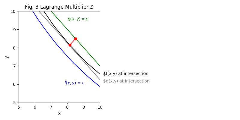
But if we need a constraint, then we need the Lagrange Multiplier. The Lagrange Multiplier is the distance (magnitude) between the point of intersection and the point dictated by \(g(x,y)\) the constraint.
A.5.2 Practical
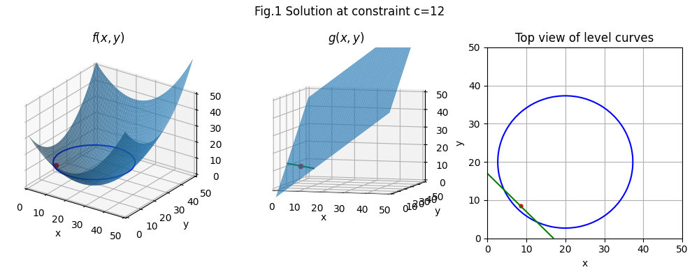
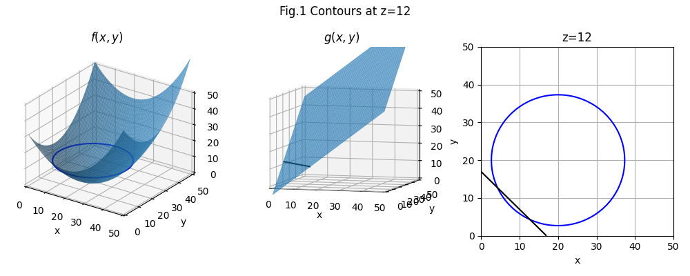
Let us take the function and constraints: $$\begin{aligned} f(x,y) &= {{(x-20)^2}\over{25}} + {{(y-20)^2}\over{25}} \\ g(x,y) &= x + y - 5 = 12 \end{aligned}$$
 What is the minimum of \(f(x,y)\), constrained by \(g(x,y)\)?
We find out by setting the gradient vector of the Lagrangian Function to 0 and determining the value of the Langrange Multiplier \(\color{green}{\lambda}\).
- The Lagrangian Function is: $$\mathcal{L}(x, y, \lambda) = f(x,y) - \color{green}{\lambda}(g(x,y)-c)$$
- The gradient vector of the Lagrangian Function is: $$ \color{red}{\triangledown}\mathcal{L}(x,y,\lambda)=\color{red}{\triangledown[}f(x,y) - \color{green}{\lambda}(g(x,y)-c)\color{red}{]} $$
- Set \(\triangledown\mathcal{L}(x,y,\lambda) = 0\) because level curves have gradient 0: $$ \langle 0,0,0 \rangle = \triangledown{[f(x,y) - \color{green}{\lambda}(g(x,y)-c)]} $$
To find all three variables λ, x, and y, we solve the system of partial derivatives (called the critical points). So let’s punch in those functions from above:
$$\begin{aligned} \begin{vmatrix}0 \\ 0 \\ 0 \end{vmatrix}&=\begin{vmatrix}f_x({1\over25}[(x-20)^2 + (y-20)^2]-\lambda(x + y -5-12))\\f_y({1\over25}[(x-20)^2 + (y-20)^2]-\lambda(x + y -5-12))\\f_\lambda({1\over25}[(x-20)^2 + (y-20)^2]-\lambda(x + y -5-12))\end{vmatrix}\\ \begin{vmatrix}0 \\ 0 \\ 0 \end{vmatrix}&=\begin{vmatrix} 0.08x - \lambda \\ 0.08y - \lambda \\ -x-y+5 \end{vmatrix} \\ \lambda&=0.08(x)\\ \lambda&=0.08(y)\\ \therefore x&=y = {17\over2} = 8.5\\ \lambda&=0.68 \end{aligned}$$ The point at the minimum is \(\langle{8.5,8.5}\rangle\).
A.5.3 Optimization
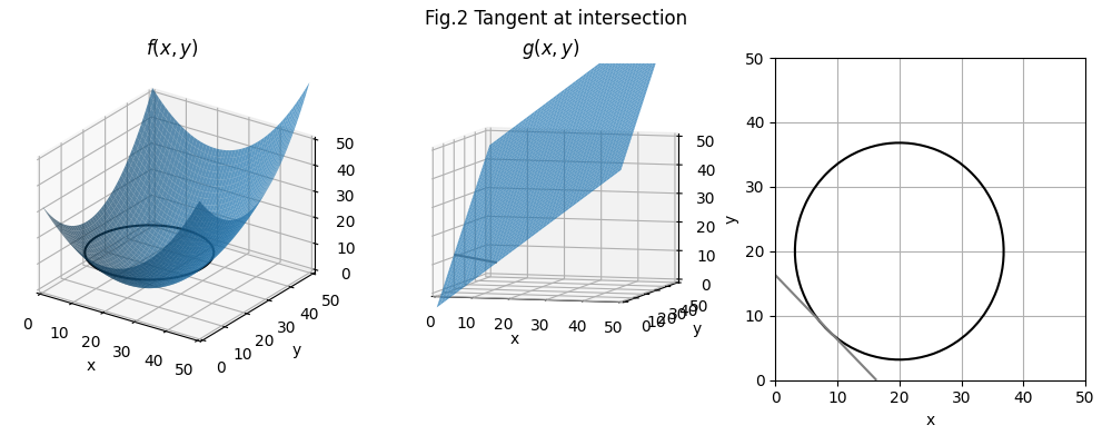
To optimize, one subtracts the Lagrange Mutiplier \(\mathcal{L}\) from the constraint. In the case where \(c=12\) and \(\mathcal{L}\) is 0.68, the optimal constraint would be 11.32, with the minimum point \(\langle{8.16,8.16}\rangle\). See Fig. 2 above.