Classification
Classification is the supervised attempt to determine if something belongs to one group or another. For example, is the email I received five minutes ago a phishing attempt or is it legit? Is the family at 123 Dunno Court, Ste-Clotilde-de-Rubber-Boot more likely to vote Bloc, Liberal or PC?The three classification methods discussed in MMAI863 are:
- KNN
- Logistic Regression
- Discriminant Analysis
KNN: K-Nearest Neighbours
Say you have two independent parameters, longitude and latitude. The dependent variable is taken from the set of the political parties: [Liberal, PC, NDP, Bloc].
The hyperparameter (user-supplied parameter) is K, a positive integer.
KNN Classification
To determine what party the citizen at \(x_0\) voted for:
- Identify the K number of points of training data closest to \(x_0\). These points are collectively known as \(N_0\).
- Estimate the conditional probability for the political party under question from the number of points in \(N_0\) whose response values were that political party.

Say j is a political party taken from [Liberal, PC, NDP, Bloc]. The conditional probabilities are calculated thus: $$ Pr(Y=j|X=x_0) = {1\over{K}}{\sum_{i\in{N_0}}}I(y_i=j)\\ I = \begin{cases} 1, & \text{if}\ y_i=j \\ 0, & \text{if}\ y_i\neq{j} \\ \end{cases} $$ This formal equation is not as evil as it looks. It merely encodes some good sense:
Say we set K to 5. If for example, two of the five citizens in the training set closest to citizen \(x_0\) voted Liberal and three voted PC, then the probabilities that the citizen at point \(x_0\) voted for each party is:
| Party | Probability |
|---|---|
| Liberal | \(2\over5\) |
| PC | \(3\over5\) |
| NDP | 0 |
| Bloc | 0 |
The good citizen at \(x_0\) probably voted PC but that’s pretty fuzzy. K is pretty small.
What is good for \(x_0\) is just as good for some other point \(x_1\). Find the closest K training points to \(x_1\) to make up \(N_1\) and apply the equation.
The K hyperparameter: inflexibility vs overtraining
The line between the points that voted for one party and the points that voted for another is called the decision boundary. It is quite frankly fuzzy, but a line needs to be drawn somewhere.
The larger the K, the less flexible the decision boundary, approaching linear (low-variance, high-bias). Conversely, the smaller the K, the more flexible the decision boundary to the point of overtraininig (high-variance, low-bias).
KNN Regression
KNN-Regression tries to estimate the function defining a linear decision boundary. The formula is:
$$ \hat{f}(x_0) = {1\over{K}}\sum_{x_i\in{N_0}}y_i $$
Logistic Regression
Logistic Regression estimates the probability (between 0 and 1) of an event occurring based on a history of odds as a linear equation.
Introducing Log Odds
Odds are the ratio of something happening vs something not happening. It is not the same as probability. If the ratio is skewed enough (e.g., me winning the lottery vs not winning), the magnitude is just too large and will screw up machine learning. Log odds, or natural logarithm of odds, is a logit function transforming a ratio to keep the magnitude reasonable:
$$ p(x) = {1\over{1 + e^{-x}}} $$
Say the odds of me winning the lottery are 1 in 13,983,816, that is x = 0.0000000715. Calculating the log odds, \(p(0.0000000715) = {1\over{1 + e^{-0.0000000715}}} = 0.500\).
For further notes, see WHAT and WHY of Log Odds.
Logistic Regression Formulae
Say making my family angry with me is only a function of my spending habits.1 Reducing their degree of anger (annoyance, frustrated, mad, incandescent) to a mere 1|0 proposition (angry/not angry) the chances of their being angry with me increases the more I spend over budget, and is reduced by the more money I save.
The shape of the simple log odds p(x) above with \(\infty < x < \infty\) forms a sigmoid curve. If I used it to determine anger as a function of my blowing the budget, we would get the following curve:
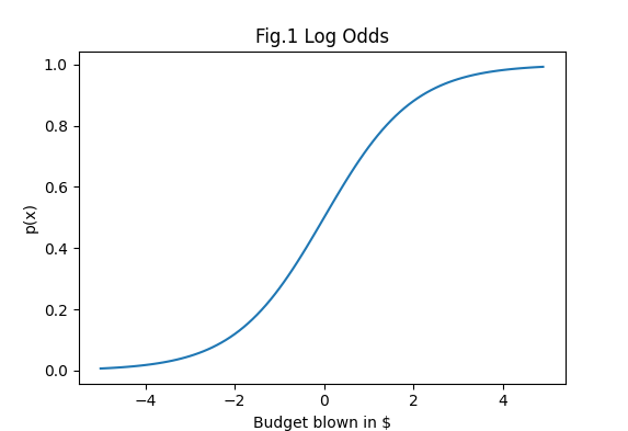
The interpretation is as follows: if I spend just as much as I brought home this month, so my net is $0.00, it’s even odds that my family will be mad with me. If I saved $500 (-5 on the scale), it’s quite clear they won’t be angry (p[-5] = 0.0067). If I spent too much on my computer habits to the tune of blowing $1000 over budget, it’s guaranteed that I’m eating my next meal on the roof (p[10] = 0.9999).
However, one cannot use the simple log odds equation for people’s behaviour! We would need to record their anger over different spending results. Say one month I was $50 under budget and they were mad at me. The next month I blew $300 and they were not. The next month +$250 set my ears ringing. The next month I saved $400 and you could feel the glow a kilometer away.
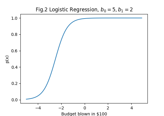
The sigmoid curve needs to be adjusted to fit the data, which means using logistic regression, not the log odds. The formula for logistic regression on one dependent variable (x) is:
$$ p(x) = {{e^{\beta_0+\beta_1x}}\over{1 + e^{\beta_0+\beta_1x}}} $$
Say we estimated from past behaviour that \(\beta_0=5, \beta_1=2\). What happends if this month I saved a paltry $100? Punching in the formula, the probability of my family being unhappy with me is 0.95. Tough crowd! In reality, my family is usually cool with me so don’t read too much into this.
Maximum Likelihood Estimation
How do we calculate each \(\beta\)?
One uses maximum likelihood estimation (MLE). To understand MLE, one needs to know what a likelihood function is. The likelihood function calculates the probability of an observed outcome given a hyperparameter \(\beta\).
For the single independent problem we have been working on, the likelihood function for any given observation is:
$$ L(\beta,y,x) = p(x\beta)^{y}[1-p(x\beta)]^{1-y} $$
where \(p(t) \) is the log odds function, \({1\over{1 + e^{-t}}} \)
For a series of observations, the likelihood function is:
$$ L(\beta,y_i,x_i) = \prod^n_{i=1}p(x_i\beta)^{y_i}[1-p(x_i\beta)]^{1-y_i} $$
The MLE maximizes the likelihood function, i.e. it sets \(\beta\) to the highest possible value that fits the data.
See Christoph M’s logistics.
See also Arun Addagatla.
Linear and Quadratic Discriminant Analysis
Linear means “using a line”. Discriminant means “discriminating factor between classes” (i.e. the decision boundary). Quadratic means “something that pertains to squares”.
Look at the following:
- Video: Stanford Online 4.5 Discriminant Analysis
- A YouTube video for LDA: https://youtu.be/2EjGJXzsC2U
- Another, from Victor Lavrenko, start at 3:54.
- https://www.knowledgehut.com/blog/data-science/linear-discriminant-analysis-for-machine-learning
- https://www.geeksforgeeks.org/ml-linear-discriminant-analysis/
Some take-home points:
Discriminant Analysis
Given the training data Pr(X|Y), model the distribution of X in each of the classes separately, then, if the data has a normal (Gaussian) distribution, use Bayes’ Rule to obtain Pr(Y|X).
Review Bayes’ Rule. Swapping out A’s and B’s for Y’s and Z’s:
$$ P(Y|X) = {{P(Y)P(X|Y)}\over{P(X)}} $$
Bayes’ Rule is rewritten differently for DA:
$$ Pr(Y=k|X=x) = {{\pi_kf_k(x)}\over{\Sigma^K_{i=1}\pi_if_i(x)}} $$
Read: “Given X, what is the probability that Y is in class k?”
- \(\pi_k\) is the prior probability for class k, i.e. \(P(Y=k)\). Obviously we get this from the training data.
- \(f_k(x)\) is the density for X in class k, i.e. \(P(X=x|Y=k)\). Also taken from the training data.
- \(\Sigma^K_{i=1}\pi_if_i(x)\) is the marginal probability \(P(X=x)\). Likewise.
The decision boundary lies where the downward probability curve of one class intersects the upward curve of another.
How LDA and QDA work
Discriminant Analysis itself doesn’t work well if the normal distributions of each class are too intermingled: the variances are wide or the distance between the maximum densities (ie the top of the curves) is too small. Enter LDA and QDA.
Linear and Quadratic Discriminant Analysis project the training data onto a smaller set of new dimensions by transforming their values in matrix form by a vector (a single row matrix). The vector is determined through a cost function: the square of the distance between each class divided by the variances of each class (i.e, how tight the classes are):
$$ \max{(u_1 - u_2)^2\over(\sigma_1^2+\sigma_2^2)} $$
where
- \(u_1 - u_2\) is the distance between the maximum densities of each class, i.e., the tops of their respecitve probability curves. You want this as far as possible.
- \(\sigma\) are the variances for each class. i.e. how the width of the curves. You want these as small as possible.
Victor Lavrenko’s video has a nice diagram of this at 4:25. Performing LDA itself can be found in Dr Sebastian Raschka’s article.
LDA vs QDA
- LDA uses a common covariance matrix (i.e., the vector) among the classes.
- QDA uses a covariance matrix per class.
Advantages and Limitations
- LDA beats logistic regression if the classes are well-separated, as LR gets weirder the more separated the classes are.
- LDA works even if the number of features is much larger than the number of training samples.
- It can handle multicollinearity.
- It cannot handle non-Gaussian distribution well, so when preparing data, try to remove outliers and deal with skewed distributions.
- High-dimension feature spaces reduce the effectiveness of LDA.
-
This is not the case, so shh. ↩︎