The Curse of Dimensionality

Mon, Oct 16, 2023 A.I. loves data! Mounds of it. Data, data, data, … except it is better to have huge rows of data and not so much columns of data. The curse of dimensionality means that the more features $x_0, x_1, …, x_n$ you have in your dataset, the more problems you will have processing them.

Some problems associated with a large number of features are:

Each feature requires more processing power and time
The distance between each data point increases with each added dimension
More features increases the risk of overfitting.

One can combine two or more features that are correlated into just one feature, or one can simply eliminate the features that have the least benefit to the machine learning algorithm.

Here are two reduction techniques.

Orthogonal Projection

Orthogonal:

From Oxford Languages:

of or involving right angles; at right angles.
in statistics, (of variates) statistically independent.

If two or more features have a linear relationship, one can simply project that data onto a plane, line, or curve using the closest vector property.

fig1

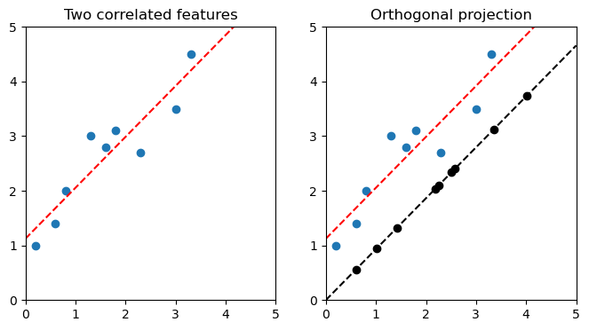
Figure 1. Correlated features with a linear relationship and their projection

Take a two-dimensional feature space, as usual, with the data scattered around the space. Create a line W, such as one created through linear regression. For each data point u, find the point on W measured from the origin closest to u. Record the lengths along W as a new, one-dimensional feature.

If the relationship is based on curves instead of linear relationships, then one resorts to neural networks.

Generalization

The original $R^x$-dimension feature set is called p-dimension. The mapped $R^{x-1}$ dimension feature set is called the manifold, or m-dimension. The transformation function from higher to lower dimensions is called the auto-encoder. The auto-encoder embeds the p-dimensional data to the closest points in the manifold.

Vectors

Remember from basic calculus, a vector describes a line segment with direction and length (magnitude). It can be represented as a variable with a right-facing arrow: $\vec{a}$. Using matrix arithmetic, it is a single column with as many rows as dimensions:

$$ \vec{a} =
\begin{bmatrix}1\\1\end{bmatrix} i.e., \text{: one unit right and one unit up in a 2D plane.}\\ \vec{b} =
\begin{bmatrix}-2\\1\end{bmatrix} i.e., \text{: two units left and one unit up in a 2D plane.} $$

fig 2

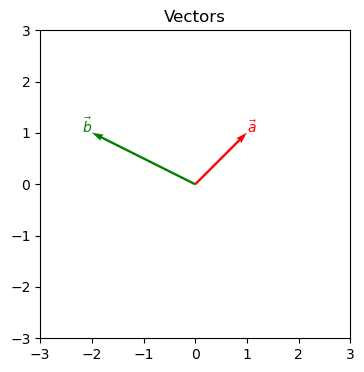
A vector does not describe position.

The Formal Definition of Orthogonal Projections:

If W is a subspace of the feature set $R^n$ and u is a vector in the feature set, the vector closest to u on W is the orthogonal projection $U_w(u)$.

To calculate $U_w(u)$, one needs the vector v of subspace W: $U_w(u) = {{v\cdot{u}}\over{v\cdot{v}}}v$

In the case of figure 1 above, the linear equation for the regression is $y = 0.93x + 1.12$. Its vector $\vec{v}$ is therefore $\begin{bmatrix}1\\0.93\end{bmatrix}$.

Example: Given the point (2.3, 2.7), what would be the orthogonal projection?

$$ \begin{array}{ll} U_w(u) &= {{v\cdot{u}}\over{v\cdot{v}}}v\\ &= { {\begin{bmatrix}1\\0.93\end{bmatrix}\cdot \begin{bmatrix}2.3\\2.7\end{bmatrix} }\over {\begin{bmatrix}1\\0.93\end{bmatrix}\cdot \begin{bmatrix}1\\0.93\end{bmatrix} } }\begin{bmatrix}1\\0.93\end{bmatrix}\\ &= {{2.3 + 2.51}\over{1 + 0.86}}\begin{bmatrix}1\\0.93\end{bmatrix}\\ &= {2.59}\begin{bmatrix}1\\0.93\end{bmatrix}\\ &= \begin{bmatrix}2.59\\2.41\end{bmatrix}\\ \end{array}\\ $$

Here is some Python code that does the same thing, without reducing to two decimal points:

import numpy as np

def orth_proj(v, u):
    """u are the vectors being projected onto v"""
    return np.dot((np.dot(u, v) / np.dot(v, v)), v)

print(orth_proj((1, 0.93), (2.3, 2.7)))
[2.57976299 2.39917958]

The orthogonal projection of point (2.3, 27) on vector (1, 0.93) is (2.58, 2.40). You can confirm point=(2.58, 2.40) on figure 1 above.

PCA

A more sophisticated technique, the principal component analysis autoencoder, replaces features with new features based on the variance of the data. It is based covariance matrixes, eigenvectors, and eigenvalues. PCA is considered an unsupervised machine learning technique.

PCA isn’t all that useful on two-dimensional sets, but it is tremendously useful on large and immense sets, when most noise can be eliminated. PCA can be used for image compression as well as signal processing, which can have a lot of information.

PCA, by the way, is closely related to the LDA discussed in classification.

This is the algorithm:

Standardize features to a mean of 0 and variance of 1. Basically, prevent different magnitudes from having influence.
Identify correlations among features through a covariance matrix.
Create uncorrelated principal components from the covariance matrix (NOT the feature data directly). This means calculating eigenvectors and eigenvalues from the covariance matrix, and then sorting them in order of eigenvalue.
Discard one or more of the lowest-value eigenvectors. The remain eigenvectors make new features by recording their dot-products on the original data.

I will delve only into some of the above.

Create the Uncorrelated Principal Components

There are as many principal components as dimensions in a feature set, in diminishing order of variance. The user decides how many components are discarded in the dimensionality reduction.

The principal components of a two-dimensional feature set are:

Principal Component 1 is the vector that corresponds to the length and direction of the greatest variance in the data as determined in the covariance matrix. This vector is one of the eigenvectors of the covariance matrix.
Principal Component 2 is the vector orthogonal (i.e. at right angles) to Principal Component 1. Being orthogonal, it is by definition uncorrelated to the above. Since it is the last component in this 2-component set, it has no variance and is generally discarded when PCA is being used for dimensionality reduction.

Eigenvectors and Eigenvalues

An eigenvector to a matrix is a non-zero vector that, when multiplied by its matrix, only changes its scale, never its direction. The eigenvalue is the scale degree that makes the eigenvector and its matrix equal.

Note that the matrix must be a square matrix, i.e. the number of rows equals the number of columns. A covariance matrix, for example, is just perfect.

Question: Is $\begin{bmatrix}3\\5\end{bmatrix}$ an eigenvector of $\begin{bmatrix}1 & 3\\2 & 4\end{bmatrix}$?

Let $\vec{a} = \begin{bmatrix}3\\5\end{bmatrix}$ and $\vec{b}$ be the product of the matrix multiplication.

$$ \begin{bmatrix} 1 & 3\\ 2 & 4 \end{bmatrix} \times \begin{bmatrix} 3\\5 \end{bmatrix}= \begin{bmatrix} 18\\ 26 \end{bmatrix} $$

fig 2

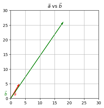
$\begin{bmatrix}3\\5\end{bmatrix}$ is not an eigenvector of $\begin{bmatrix}1 & 3\\2 & 4\end{bmatrix}$. When it is multiplied with the matrix, its direction changes.

Find the Eigenvector

There may be more than one eigenvectors to a given matrix. To find the eigenvectors, first find the eigenvalues, i.e. the scale degree. The definition of an eigenvector is:

A nonzero vector v is an eigenvector of matrix A if there exists a scalar $\lambda$ so that $A\vec{v} = \lambda\vec{v}$. This means that one finds $\lambda$ so that $Av - \lambda{v} = 0$.

In other words, $\lambda$ is the eigenvalue.

$$ \begin{array}{ll} \begin{bmatrix} 1 - \lambda & 3\\ 2 & 4 - \lambda \end{bmatrix} &= 0\\ (1 - \lambda)(4 - \lambda) - (3)(2) &= 0\\ 4 - \lambda - 4\lambda + \lambda^2 - 6 &= 0\\ \lambda^2 -5\lambda - 2 &= 0\\ \end{array} $$

… and so on. Actually finding the possible values of $\lambda$ and their appropriate vectors v can be painful by hand, so we’ll just leave it to the computer:

import numpy as np
from numpy.linalg import eig
matrix = np.array([[1,3],
                   [2,4]])
eigenvalues, eigenvectors = eig(matrix)
print(eigenvalues)  # Can only go so many decimal points
[-0.37228132  5.37228132]

print(eigenvectors)
[[-0.90937671 -0.56576746]
 [ 0.41597356 -0.82456484]]