Linear Regression
Linear regression is an umbrella term for the simplest machine learning algorithms. Used in supervised learning, it works only if there is a linear relationship between inputs X and their dependent variables Y.Recall that a line equation is \(y=mx+b\). m and b (aka \(\beta_1\) and \(\beta_0 \) respectively), are the parameters. The point of machine learning here is to find a close estimate of the parameters given training values of X and Y.
Ordinary Least Squares
Rarely will \((x_0, y_0),(x_1, y_1),(x_2, y_2)\) in a real-life scenario be exactly on the same line defined by \(y=mx+b\). There will always be some unavoidable error \(\epsilon\). The idea of OLS is to find values for \([m, b]\) that minimize the effect of the errors.
RSS
The calculation used to determine the collective effect of the errors is called RSS: Residual Sum of Squares.
$$ RSS={\sum^n_{i=1}}(y_i-\hat\beta_0-\hat\beta_1x_i)^2 $$
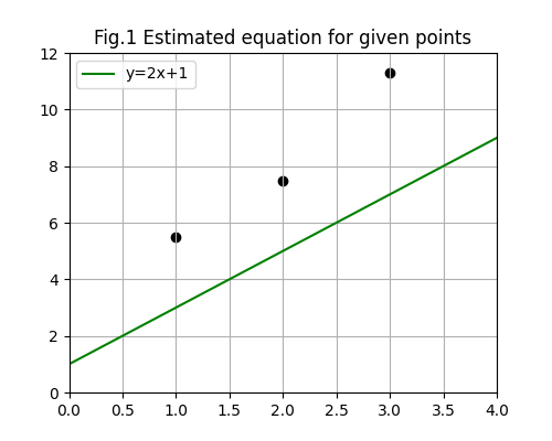
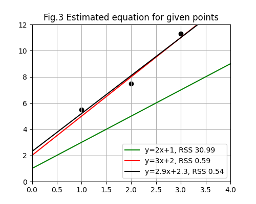
Say we have the training set {(1, 5.5), (2, 7.5), (3, 11.3)}. If we guess that m is 2 and b is 1, we would get the RSS as such:
$$
(5.5-1-2(1))^2+(7.5-1-2(2))^2+(11.3-1-2(3))^2 = 30.99
$$
If we think that m is 3 and b is 2:
$$
(5.5-2-3(1))^2+(7.5-2-3(2))^2+(11.3-2-3(3))^2 = 0.59
$$
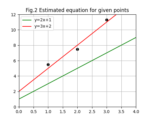
We see that \(y=3x+2\) is a much more accurate guess of the linear equation describing the training set.
OLS Equation
The equations that automagically finds OLS using RSS as a measure are:
$$\begin{aligned} \hat{m} &= {{\sum^n_{i=1}(x_i-\bar{x})(y_i-\bar{y})}\over{\sum^n_{i=1}(x_i-\bar{x})^2}}\\ \hat{b} &= \bar{y}-\hat{m}\bar{x} \end{aligned}$$
These equations were made when taking the first derivatives with respect to m and b and making them equal to zero. Look it up.
Taking the same training data as above, we calculate m:
$$\begin{aligned} \hat{m} &= {{\sum^n_{i=1}(x_i-\bar{x})(y_i-\bar{y})}\over{\sum^n_{i=1}(x_i-\bar{x})^2}}\\ \bar{x} &= (1+2+3)/2=2\\ \bar{y} &= (5.5+7.5+11.3)/3=8.1\\ \hat{m} &= {{(1-2)(5.5-8.1)+(2-2)(7.5-8.1)+(3-2)(11.3-8.1)}\over{(1-2)^2+(2-2)^2+(3-2)^2}}\\ \hat{m} &= {{2.6+3.2}\over2}=2.9 \end{aligned}$$
And to calculate b:
$$\begin{aligned} \hat{b} &= \bar{y}-\hat{m}\bar{x}\\ \hat{b} &= 8.1-2.9(2) = 2.3 \end{aligned}$$
The equation estimates the line equation as \(y=2.9x+2.3\).
This works only if errors \(\epsilon_1, \epsilon_2, …, \epsilon_n\)
- Are independent from run to run
- Have zero mean and are normally distributed (i.e, not skewed)
- Little to no multicollinearity
- Are homoscedastic (the variances in different groups being compared are similar).
… and of course assuming that X and Y have a linear relationship.
Explanability
If we want to know how much of the variability of Y is explained by X (i.e. how much are the changes in the set Y explained by the changes in X), we calculate \(R^2\), the coefficient of determination. \(R^2=1-{{RSS}\over{TSS}}\), where TSS is the total sum of squares of Y, and RSS (residual sum of squares) is the sum of the squares of the errors, \(\epsilon\), just as explained above.
$$\begin{aligned} TSS &= {\sum^n_{i=1}(y_i-\bar{y})^2}\\ RSS &= {\sum^n_{i=1}(y_i-\hat{y_i})^2} \end{aligned}$$
Using the same training set {(1, 5.5), (2, 7.5), (3, 11.3)}, we calculate:
$$\begin{aligned} TSS &= (5.5-8.1)^2 + (7.5-8.1)^2 + (11.3-8.1)^2 = 17.36\\ RSS &= (5.5-5.2)^2 + (7.5-8.1)^2 + (11.3-11.0)^2 = 0.54\\ R^2 &= 1 - {{0.54}\over{17.36}} = 0.969 \end{aligned}$$
Yes, but is this good? According to Wikipedia, a perfect fit is \(R^2 = 1\). The baseline, which will always predict the mean of y (i.e., \(\bar{y}\)) is \(R^2=0\).
RSS for more than two dimensions
If the data is multivariate, the equations change. \(y=mx+b\) has a general form, \(c=ax+by\). Since the general form of a three-dimensional linear equation is \(d=ax+by+cz\), and fourth is \(e=ax+by+cz+dwhatever\) we can forgo the alphabet and use \(\beta\) for the coefficients and x for the independent variables instead even though it sucks typing \beta all the time in LaTeX: \(\beta_0=\beta_1x_1+\beta_2x_2+…+\beta_px_p\). We can use y for the dependent variable: \(y=\beta_0+\beta_1x_1+\beta_2x_2+…+\beta_px_p\).
The RSS is now:
$$ RSS = {\sum^n_{i=1}}(y_i-\beta_0-\sum^p_{j=1}\beta_{j}x_{ij})^2 $$
n of course is the number of instances, whereas p is the number of dimensions.
This sucker doesn’t use the OLS equation derived from the first derivatives mentioned above. This one will need convex optimization. This I will discuss next post.